Alchemical Transfer Method

In this tutorial, you will use BioSimSpace to set up and run a Relative Binding Free Energy (RBFE) calculation using the alchemical transfer method (ATM) on a pair of ligands bound to Tyrosine kinase 2 (TYK2).

Note

ATM calculations are currently only available in OpenMM. As such, an environment containing OpenMM is required to run this tutorial.

This tutorial assumes that you are familiar with the concepts of the Alchemical Transfer Method. If you are not, please see the Gallichio lab website as well as the corresponding publications for an in-depth explanation of the method, as well as the intricacies involved in setting up an ATM calculation.

System Setup

Import BioSimSpace using:

>>> import BioSimSpace as BSS

Now load the set of example molecules from a URL, via BioSimSpace.IO.readMolecules():

>>> url = BSS.tutorialUrl()
>>> protein = BSS.IO.readMolecules([f"{url}/tyk2.prm7", f"{url}/tyk2.rst7"])[0]
>>> lig1 = BSS.IO.readMolecules([f"{url}/ejm_31.prm7", f"{url}/ejm_31.rst7"])[0]
>>> lig2 = BSS.IO.readMolecules([f"{url}/ejm_43.prm7", f"{url}/ejm_43.rst7"])[0]

In order to run an ATM calculation, a single system containing both ligands and the protein in their correct positions is needed. This can be created using functionality provided in BioSimSpace.FreeEnergy.ATMSetup().

ATM calculations require that both ligands be present in the system simultaneously, with one ligand bound to the receptor and the other free in the solvent. As such, the first decision to be made when setting up an ATM calculation is which ligand will be bound and which will be free.

It is important to note that, while one ligand is chosen to be bound, both ligands will bound to the receptor at some point during the calculation, the choice made here simply defines the initial state of the system, and by extension the direction of the calculation.

The first step in creating an ATM-compatible system in BioSimSpace is to create an ATMSetup object, which will be used to prepare the system:

>>> atm_setup = BSS.FreeEnergy.ATMSetup(receptor=protein,
...     ligand_bound=lig1,
...     ligand_free=lig2
... )

Before an ATM-ready system can be prepared there are decisions to be made regarding the system setup, namely which atoms will be used to define the rigid cores of the ligands, as well those that make up the centre of mass of each molecule.

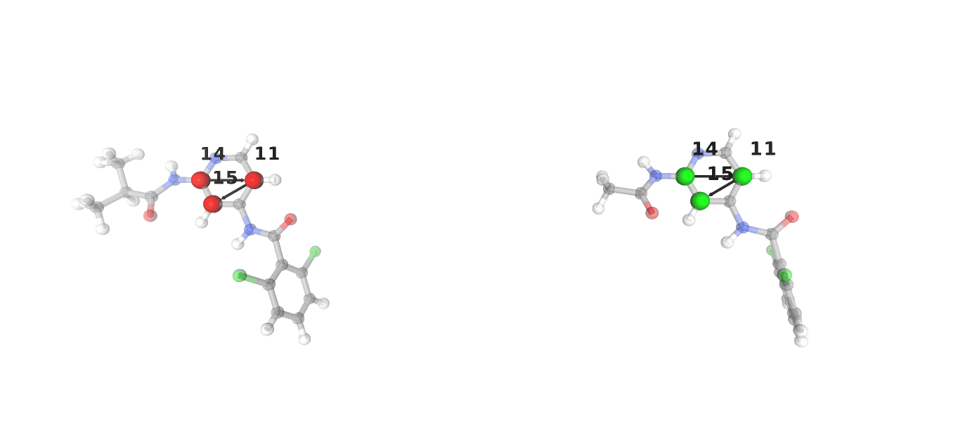
The choice of rigid core atoms is vital to the success of an ATM RBFE calculation, and as such BioSimSpace provides a helper function to visualise the choice made by the user.

>>> BSS.FreeEnergy.ATMSetup.viewRigidCores(
...     ligand_bound=lig1,
...     ligand_free=lig2,
...     ligand_bound_rigid_core=[14, 11, 15],
...     ligand_free_rigid_core=[14, 11, 15]
... )

Note

In this case the choice of rigid core atoms is the same for both ligands, but this is not always the case. The choice of these atoms should be made on a ligand to ligand basis.

For help in choosing the correct atoms, see the Gallichio lab tutorial.

Now that a sensible choice of rigid core atoms has been made, there are a few more choices to be made before the system can be prepared. The most important of these is the choice of displacement vector, which defines the direction and distance at which the free ligand will be placed relative to the bound ligand. It is generally recommended that this displacement be at least 3 layers of water molecules (> 10 Å) thick. If no displacement is provided BioSimSpace will find a best guess translation vector based on the relative positions of the protein and bound ligands and translate the free ligand 20Å along this vector.

This is also the point at which a custom set of atoms can be chosen to define the centre of mass of both the ligands and the protein. In the majority of cases it should not be necessary to change the default choice of atoms, but the option is there if needed and can be set using the ligand_bound_com_atoms and ligand_free_com_atoms arguments.

Now that all the choices have been made, the system can be prepared:

>>> system, atm_data = atm_setup.prepare(
...     ligand_bound_rigid_core=[14, 11, 15],
...     ligand_free_rigid_core=[14, 11, 15]
... )

The prepare function returns a pair of objects, the first is the prepared protein-ligand-ligand system, and the second is a dictionary containing the choices made during the setup process. This atm_data object will be passed to protocols for minimisation, equilibration and production in order to ensure that options chosen during setup are properly carried through.

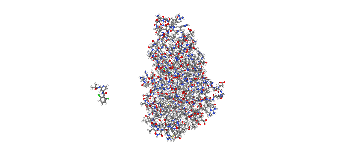
The prepared system can be visualised using BioSimSpace’s built in visualisation functionality:

>>> v = BSS.Notebook.View(system)
>>> v.system()

Now all that remains is to solvate the system.

>>> solvated = BSS.Solvent.tip3p(molecule=system, box=3 * [7 * BSS.Units.Length.nanometer])

Minimisation and Equilibration

Now that the system is fully prepared, the next step is to minimise and equilibrate. The minimisation and equilibration of systems using alchemical transfer is more complex than standard systems, and is a multi-stage process.

First, if positional restraints are needed, which is generally recommended for ATM calculations, the decision of which atoms to restrain must be made. A good choice for these atoms are the alpha carbons of the protein. These can be found using BioSimSpace search syntax:

>>> ca = [atom.index() for atom in solvated.search("atomname CA")]

The system can now be minimised. Unlike standard minimisation, the minimisation of an ATM system requires that several restraints be applied from the start. These restraints are: core alignment, applied to atoms determined earlier, which can be turned on or off by passing the core_alignment argument; positional restraints applied to the alpha carbons listed above, set using the restraint argument; and a centre of mass distance restraint, which maintains the distance between the centre of masses of the ligands, as well as the distance between the centre of mass of the protein and ligands, set using the com_distance_restraint argument. The strength of these restraints is automatically set to a set of default values that are generally suitable for most systems, but can also be set manually by passing the relevant arguments to BioSimSpace.Protocol.ATMMinimisation:

>>> minimisation = BSS.Protocol.ATMMinimisation(
...     data=atm_data,
...     core_alignment=True,
...     restraint=ca,
...     com_distance_restraint=True
... )

This minimisation protocol can now be run as a standard BioSimSpace OpenMM process:

>>> minimisation_process = BSS.Process.OpenMM(solvated, minimisation)
>>> minimisation_process.start()
>>> minimisation_process.wait()
>>> minimised = minimisation_process.getSystem(block=True)

Now the first stage of equilibration can be run. Similar to the minimisation, this protocol has several restraints that are applied from the start:

>>> equilibration = BSS.Protocol.ATMEquilibration(
...    data=atm_data,
...    core_alignment=True,
...    restraint=ca,
...    com_distance_restraint=True,
...    runtime="100ps"
... )
>>> equilibrate_process = BSS.Process.OpenMM(minimised, equilibration, platform="CUDA")
>>> equilibrate_process.start()
>>> equilibrate_process.wait()
>>> equilibrated = equilibrate_process.getSystem(block=True)

Note

The equilibration protocol is set to run for 100ps. This is a relatively short time, and should be increased for production runs.

Here the “CUDA” platform is explicitly set. It is highly recommended to use a GPU platform for equilibration and production runs, as the calculations are computationally expensive.

Now that the system has been minimised and equilibrated without the ATMForce present, it needs to be added to the system. The first stage of this introduction is annealing, which by default will gradually increase the value of λ from 0 to 0.5 over a number of cycles:

>>> annealing = BSS.Protocol.ATMAnnealing(
...    data=atm_data,
...    core_alignment=True,
...    restraint=ca,
...    com_distance_restraint=True,
...    runtime="100ps",
...    anneal_numcycles=10
... )
>>> annealing_process = BSS.Process.OpenMM(equilibrated, annealing, platform="CUDA")
>>> annealing_process.start()
>>> annealing_process.wait()
>>> annealed = annealing_process.getSystem(block=True)

The annealing process is fully customisable, and any number of λ-specific values can be annealed. See BioSimSpace.Protocol.ATMAnnealing for full the full list of annealing options.

The final stage of the ATM minimisation and equilibration protocol is a post-annealing equilibration run, this time with the ATMForce present at λ=0.5:

>>> post_anneal_equilibration = BSS.Protocol.ATMEquilibration(
...    data=atm_data,
...    core_alignment=True,
...    restraint=ca,
...    com_distance_restraint=True,
...    use_atm_force=True,
...    lambda1 = 0.5,
...    lambda2 = 0.5,
...    runtime="100ps"
... )
>>> post_anneal_equilibration_process = BSS.Process.OpenMM(
...     annealed,
...     post_anneal_equilibration,
...     platform="CUDA"
... )
>>> post_anneal_equilibration_process.start()
>>> post_anneal_equilibration_process.wait()
>>> min_eq_final = post_anneal_equilibration_process.getSystem(block=True)

Note

A frequent source of instability in ATM production runs is an overlap between the bound ligand and the protein after a swap in direction. If this is encountered the first step taken should be to increase the runtime of the post-annealing equilibration. This gives the system time to adjust to the presence of the new ligand, without the reduced stability associated with a swap in direction.

Production and Analysis

The system is now ready for production. The key decision to be made before beginning is the number of lambda windows, set using the num_lambda argument. If this value is not set, a default of 22 will be set by BioSimSpace.

Note

Keep in mind that, due to the nature of the alchemical transfer method, a single production run contains both the forward and reverse direction of both the free and bound legs, and therefore a larger than usual number of lambda windows is required for a well sampled result.

In addition to setting the number of lambdas, any or all of the λ-specific values can be manually set, with the only condition being that the lists provided are all of the same length, specifically they must have length equal to num_lambda. See BioSimSpace.Protocol.ATMProduction for a full list of options.

In the case of this TYK2 perturbation, the default values for alpha and uh will need to be set manually, as the default values are not suitable.

>>> alpha = 22 * [0.1]
>>> uh = 22 * [110.0]
>>> output_directory = "tyk2_atm"
>>> production_atm = BSS.Protocol.ATMProduction(
...    data=atm_data,
...    core_alignment=True,
...    restraint=ca,
...    com_distance_restraint=True,
...    runtime = "1ns",
...    num_lambda=22,
...    alpha=alpha,
...    uh=uh,
... )
>>> production_process = BSS.FreeEnergy.ATM(
...    system=min_eq_final,
...    protocol=production_atm,
...    work_dir=output_directory,
...    platform="CUDA",
...    setup_only=True
... )

The setup_only flag is set to True here, this means that all input files will be created, but nothing will be run. It is recommended to run production protocols on HPC resources where multiple GPUs are available, as the calculations can be very computationally expensive.

Running the generated inputs is as simple as running the OpenMM.py script contained in each of the labelled lambda folders of the output directory.

Once production is complete, the results can be analysed using the built-in BioSimSpace UWHAM analysis tool.

>>> BSS.FreeEnergy.ATM.analyse(output_directory)

This will give the ΔΔG value for the perturbation, as well as the error (both in kcal/mol).

That concludes the tutorial on setting up and running an ATM RBFE calculation! For further information please visit the API documentation, and for further information on the alchemical transfer method, see the Gallichio lab website.