Hydration free energy¶

In this tutorial you’ll learn how to use BioSimSpace to set up a set of alchemical free energy simulations to compute the relative free energy of hydration ethane and methanol. Alchemical free energy calculations employ unphysical (“alchemical”) intermediates to estimate the free energies of various physical processes. Here, we will exploit a perturbation pathway between ethane and methanol which will allow us to estimate the relative free energy difference in solution, \({\Delta G_{\mathrm{sol}}}\), and vacuum, \({\Delta G_{\mathrm{vac}}}\). The free energy of hydration, \({\Delta\Delta G_{\mathrm{hyd}}}\) can then be computed from the difference between the free energy of the solvation and vacuum simulation legs, i.e.

\({\Delta\Delta G_{\mathrm{hyd}} = \Delta G_{\mathrm{sol}} - \Delta G_{\mathrm{vac}}}\)

To get started, let’s import BioSimSpace and create ethane and methanol molecules parameterised with the Generalised AMBER Force-Field (GAFF).

>>> import BioSimSpace as BSS
>>> ethane = BSS.Parameters.gaff("CC").getMolecule()
>>> methanol = BSS.Parameters.gaff("CO").getMolecule()

In order to create a perturbation between the two molecules we need to define a mapping. This mapping defines the maximum common substructure (MCS) between the molecules, mapping indices from one to the matching indices in the other. The BioSimSpace.Align package provides tools for calculating the mappings between molecules and for aligning and merging molecules based on a mapping. The user can request a multiple mappings, which can be scored and aligned in various ways. Here we’ll simply use the default options and compute the highest scoring mapping between the molecules:

>>> mapping = BSS.Align.matchAtoms(ethane, methanol)

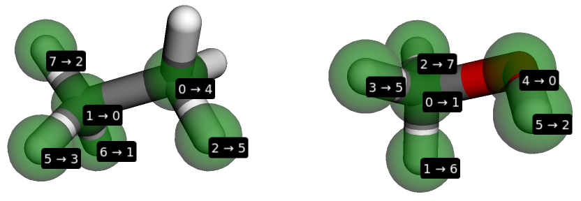
The mapping is just a dictionary mapping atoms in the ethane molecule to those in the methanol. To see what atoms have been mapped we can print the corresponding atoms from each molecule:

>>> for idx0, idx1 in mapping.items():
...     print(ethane.getAtoms()[idx0], "<-->", methanol.getAtoms()[idx1])
...
<BioSimSpace.Atom: name='H', molecule=2 index=5> <--> <BioSimSpace.Atom: name='H3', molecule=3 index=3>
<BioSimSpace.Atom: name='C', molecule=2 index=1> <--> <BioSimSpace.Atom: name='C', molecule=3 index=0>
<BioSimSpace.Atom: name='H', molecule=2 index=6> <--> <BioSimSpace.Atom: name='H1', molecule=3 index=1>
<BioSimSpace.Atom: name='H', molecule=2 index=7> <--> <BioSimSpace.Atom: name='H2', molecule=3 index=2>
<BioSimSpace.Atom: name='C', molecule=2 index=0> <--> <BioSimSpace.Atom: name='OH', molecule=3 index=4>
<BioSimSpace.Atom: name='H', molecule=2 index=2> <--> <BioSimSpace.Atom: name='HO', molecule=3 index=5>

When working running interactively, e.g. within an IPython, console or Jupyter notebook, it’s possible to visualise the mapping:

>>> BSS.Align.viewMapping(ethane, methanol, mapping)

Perturbed bonds and elements are shown in blue. Red atoms are those that are unique to a particular end state.

Mapping between atoms in ethane (left) and methanol (right) for an alchemical transformation.

Next we need to align the ethane molecule to the methane based on the mapping. The BioSimSpace.Align.rmsdAlign function will align them based on a root mean square displacement (RMSD) scoring function, whereas BioSimSpace.Align.flexAlign will flexibly align ethane to methanol using the fkcombu program, which can be useful if you want both molecules to be aligned to a specific pose. For simplicity we’ll use the RMSD alignment:

>>> ethane = BSS.Align.rmsdAlign(ethane, methanol, mapping)

Note

If we were to omit the mapping argument above, then the rmsdAlign function would compute the best mapping for us automatically. This means that we can choose to compute the mapping then align separately, or do the whole thing in one step.

Having successfully aligned the ethane molecule, we now need to merge the two molecules together to create a merged (or perturbable molecule). This contains all of the properties, e.g. bonds, angles, dihedrals, needed to define the two molecules at either end state of the perturbation, \({\lambda=0}\) and \({\lambda=1}\). The end states represent the two molecules (ethane in one state, methanol in the other) plus dummy (or virtual) atoms for any atoms from the other molecule that aren’t part of the MCS.

>>> merged = BSS.Align.merge(ethane, methanol, mapping)

Next we need to solvate our merged molecule in a box of water. Here we’ll use the TIP3P water model and a cubic box with a base length of 5 nanometers:

>>> solvated = BSS.Solvent.tip3p(molecule=merged, box=3 * [5 * BSS.Units.Length.nanometer])

Finally we can create objects to perform the perturbations for each leg of the calculation, which will automatically configure everything that is needed to run the simulations. First we will use our built in, GPU optimised, molecular dynamics engine called SOMD. (This is a wrapper around the excellent OpenMM package and is the default engine if no other packages are present.)

>>> protocol = BSS.Protocol.FreeEnergyProduction()
>>> free_somd = BSS.FreeEnergy.Relative(solvated, protocol, engine="somd", work_dir="freenrg_somd/free")
>>> vac_somd = BSS.FreeEnergy.Relative(merged.toSystem(), protocol, engine="somd", work_dir="freenrg_somd/vacuum")

Note

For GROMACS, you can use BioSimSpace.Protocol.FreeEnergyMinimisation and BioSimSpace.Protocol.FreeEnergyEquilibration to minimise and equilibrate at each \({\lambda}\) value prior to setting up to the production run above. For SOMD this isn’t possible, so you can either use GROMACS to prepare production input for each window, or use the regular BioSimSpace.Protocol.Minimisation and BioSimSpace.Protocol.Equilibration protocols to minimise and equilibrate the \({\lambda=0}\) and \({\lambda=1}\) states only using any supported engine from BioSimSpace.Process.

Note

It’s possible to use a different protocol or molecular dynamics engine for each leg, e.g. if you want to use a different \({\lambda}\) schedule.

When complete, BioSimSpace will have set up a folder hierarchy containing everything that is needed to run the hydration free energy calculation using SOMD. Let’s examine the work_dir for the free (solvated) leg specified above:

$ ls freenrg_somd
free  vacuum

Inside the top-level directory are two sub-directories called free and vacuum. These correspond the the solvated and vacuum legs of the simulation. Let’s further examine the free directory to see what’s inside:

$ ls freenrg_somd/free
lambda_0.0000  lambda_0.3000  lambda_0.6000  lambda_0.9000
lambda_0.1000  lambda_0.4000  lambda_0.7000  lambda_1.0000
lambda_0.2000  lambda_0.5000  lambda_0.800

Inside this are 11 further sub-directories, one for each of the \({\lambda}\) windows of the leg. Within each of these directories are all of the files needed to run an individual simulation, e.g.:

$ ls freenrg_somd/free/lambda_0.0000
somd.cfg  somd.err  somd.out  somd.pert  somd.prm7  somd.rst7

The BioSimSpace.FreeEnergy.Relative object can also automatically run all of the simulations for you and analyse the output that is generated. However, since these simulations will take a long time we won’t run them here.

By specifying a different molecular dynamics engine, we can use the exact same code to set up an identical set of simulations with GROMACS:

>>> free_gmx = BSS.FreeEnergy.Relative(solvated, protocol, engine="gromacs", work_dir="freenrg_gmx/free")
>>> vac_gmx = BSS.FreeEnergy.Relative(merged.toSystem(), protocol, engine="gromacs", work_dir="freenrg_gmx/vacuum")

Let’s examine the directory for the \({\lambda=0}\) window of the free leg:

$ ls freenrg_gmx/free/lambda_0.0000
gromacs.err  gromacs.mdp  gromacs.out.mdp  gromacs.tpr
gromacs.gro  gromacs.out  gromacs.top

Similarly, we can also set up the same simulations using AMBER:

free_amber = BSS.FreeEnergy.Relative(solvated, protocol, engine="amber", work_dir="freenrg_amber/free")
vac_amber = BSS.FreeEnergy.Relative(merged.toSystem(), protocol, engine="amber", work_dir="freenrg_amber/vacuum")

Let’s examine the directory for the \({\lambda=0}\) window of the free leg:

$ ls freenrg_amber/free/lambda_0.0000
amber.cfg  amber.err  amber.out  amber.prm7  amber_ref.rst7  amber.rst7

There you go! This tutorial has shown you how BioSimSpace can be used to easily set up everything that is needed for complex alchemical free energy simulations. Please visit the API documentation for further information.